Auteur: Dominique Rodriguez
Source: tangente.sty
Le code, en cours de développement (juin 2004), proposé ici permet le tracé de tangentes à des courbes quelles soient représentatives d'une fonction, paramétrées ou en coordonnées polaires.
Deux modes sont possibles : les nombres dérivés sont approchés à l'aide d'une dérivée centrale ou ils sont calculés à partir de l'expression de la dérivée.
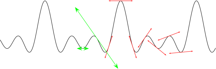
Courbe représentative d'une fonction
Approximations des nombres dérivés

\def\F{x 3.1415926 div 180 mul dup dup cos exch 2 mul cos add exch 3 mul cos add}
\psset{plotpoints=1001}
\begin{pspicture}(-10,-3)(10,3)%\psgrid
  \psplot{-10}{10}{\F}
  \psset{linecolor=red, arrows=<->}
  \psplottangent{0}{1}{\F}
  \psplottangent{1}{1}{\F}
  \psplottangent{2}{1}{\F}
  \psplottangent{3}{1}{\F}
  \psplottangent{4}{1}{\F}
  \psplottangent{5}{1}{\F}
  \psplottangent{-1}{1}{\F}
  \psset{linecolor=green, arrowscale=3}
  \psplottangent{-2}{3.14}{\F}
  \psplottangent{-3.1415926}{.5}{\F}
\end{pspicture}


Calcul à partir de la dérivée
\def\F{x 3.1415926 div 180 mul dup dup cos exch 2 mul cos add exch 3 mul cos add}
\psset{plotpoints=1001}
\def\DerivF{x 3.1415926 div 180 mul dup dup sin exch 2 mul sin 2 mul add exch 3 mul sin 3 mul add neg}
\begin{pspicture}(-10,-3)(10,3)%\psgrid
  \psplot{-10}{10}{\F}
  \psset{Derive=\DerivF, linecolor=red, arrows=<->}
  \psplottangent{0}{1}{\F}
  \psplottangent{1}{1}{\F}
  \psplottangent{2}{1}{\F}
  \psplottangent{3}{1}{\F}
  \psplottangent{4}{1}{\F}
  \psplottangent{5}{1}{\F}
  \psplottangent{-1}{1}{\F}
  \psset{linecolor=green, arrowscale=3}
  \psplottangent{-2}{3.14}{\F}
  \psplottangent{-3.1415926}{.5}{\F}
\end{pspicture}
Courbe en polaires
Approximations des nombres dérivés
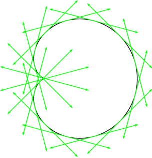
\def\Cardio{1 t cos add 2 mul}
\psset{plotpoints=1001}
\begin{pspicture}(-2,-4)(4,4)%\psgrid
  \polarplot{0}{360}{\Cardio}
  %\multido{\n=10+10}{36}{\polarplotput{\n}{\Cardio}{\pstGeonode[PointName=A_{\n}]{A_\n}}}
  \psset{linecolor=green, arrows=<->}
  \multido{\n=10+20}{18}{\polarplottangent{\n}{2}{\Cardio}}
  %\polarplottangent{180}{2}{\Cardio}
\end{pspicture}
Calcul à partir de la dérivée
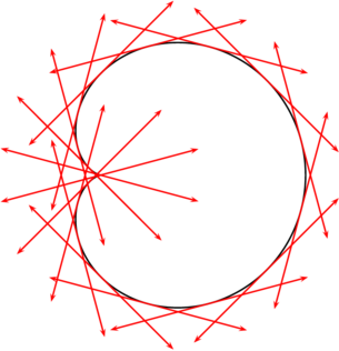
\psset{plotpoints=1001}
\def\Cardio{1 t cos add 2 mul}
\def\DerivCardio{t sin -2 mul}
\begin{pspicture}(-2,-4)(4,4)%\psgrid
  \polarplot{0}{360}{\Cardio}
  %\multido{\n=10+10}{36}{\polarplotput{\n}{\Cardio}{\pstGeonode[PointName=A_{\n}]{A_\n}}}
  \psset{Derive=\DerivCardio, linecolor=red, arrows=<->}
  \multido{\n=10+20}{18}{\polarplottangent{\n}{2}{\Cardio}}
  %\polarplottangent{80}{2}{\Cardio}
\end{pspicture}
Courbe paramétrée
Approximations des nombres dérivés
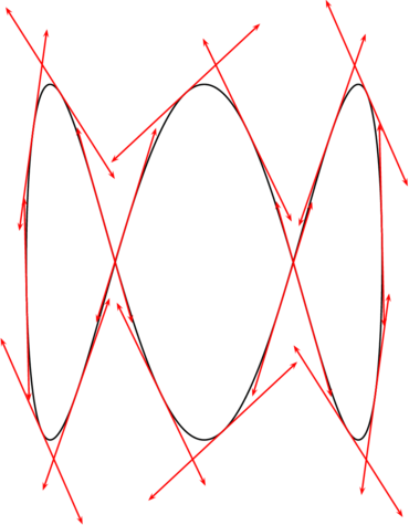
\def\Lissa{t dup 2 mul cos  3.5 mul exch 6 mul sin 3.5 mul}
\psset{plotpoints=1001}
\begin{pspicture}(-4,-4)(4,4)%\psgrid
  \parametricplot{0}{180}{\Lissa}
  %\multido{\n=2+2}{90}{\parametricplotput{\n}{\Lissa}{\pstGeonode[PointName=M_{\n}]{M_\n}}}
  \psset{linecolor=red, arrows=<->}
  %\parametricplottangent{88}{2}{\Lissa}
  \multido{\n=2+10}{18}{\parametricplottangent{\n}{2}{\Lissa}}
\end{pspicture}
Calcul à partir des dérivées
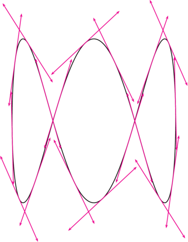
\psset{plotpoints=1001}
\def\Lissa{t dup 2 mul cos  3.5 mul exch 6 mul sin 3.5 mul}
\def\DerivLissa{t dup 2 mul sin -7 mul exch 6 mul cos 21 mul}
\begin{pspicture}(-4,-4)(4,4)%\psgrid
  \parametricplot{0}{180}{\Lissa}
  %\multido{\n=2+2}{90}{\parametricplotput{\n}{\Lissa}{\pstGeonode[PointName=M_{\n}]{M_\n}}}
  \psset{Derive=\DerivLissa, linecolor=magenta, arrows=<->}
  %\parametricplottangent{88}{2}{\Lissa}
  \multido{\n=2+10}{18}{\parametricplottangent{\n}{2}{\Lissa}}
\end{pspicture}
Exemple simple
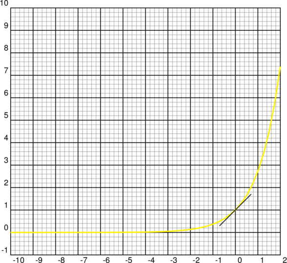
\begin{pspicture}(-10,-1)(2,10)\psgrid
  \psplot[linewidth=2\pslinewidth, linecolor=yellow]{-10}{2}{2.718 x exp}
  \psplottangent[Derive=2.718 x exp]{0}{1}{2.718 x exp}
\end{pspicture}
La compilation de ces morceaux de code nécessite l'utilisation, en plus de tangente.sty, des paquets pst-plot et pst-eucl.