Exemples de la distribution

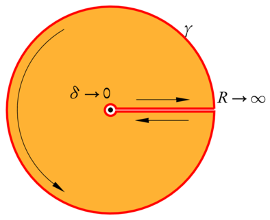
/* -*-ePiX-*- */
/* contour.c -- March 29, 2002 */
#include "epix.h"
using namespace ePiX;

int main() 
{
  bounding_box(P(-5, -5), P(5,5));
  picture(160, 160);
  unitlength("0.35mm");
  offset(100,-25);

  use_pstricks();
  begin();  degrees();
  double theta=60;
  double rad=0.25, Rad=4.5; // arc radii
  double ht=1.0/16;         // half-width of slit

  // "start" angles of arcs
  double theta1 = Asin(ht/rad), theta2 = Asin(ht/Rad);

  // build keyhole in pieces; += concatenates, -= reverses orientation
  path contour(P(0,0), Rad*E_1, Rad*E_2, theta2, 360-theta2);    // outer arc
  contour -= path(polar(rad,-theta1), polar(Rad,-theta2));       // lower slit
  contour -= path(P(0,0), rad*E_1, rad*E_2, theta1, 360-theta1); // inner arc
  contour += path(polar(rad, theta1), polar(Rad, theta2));       // upper slit

  fill();
  // raw output -- PSTricks command
  std::cout << "\n\\newrgbcolor{orange}{1 0.7 0.2}";

  psset("fillcolor=orange,linecolor=red,linewidth=1.5pt");
  contour.set_fill();
  contour.draw();
  use_pstricks(false);

  dot(P(0,0));   // the origin
  gray(1); // blacken arrowheads
  arrow(P(Rad/4, 0.1*Rad), P(3*Rad/4, 0.1*Rad)); // arrow ends in terms of Rad
  arrow(P(3*Rad/4, -0.1*Rad), P(Rad/4, -0.1*Rad));
  arc_arrow(P(0,0), 0.9*Rad, 180-theta, 180+theta);

  label(P(Rad,ht), P(2,4), "$R\\to\\infty$", tr);
  label(P(0,rad), P(0,4), "$\\delta\\to0$", tl);
  label(polar(Rad, 45), P(0,0), "$\\gamma$", tr);

  end();
}