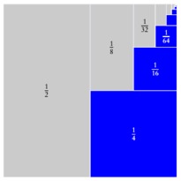
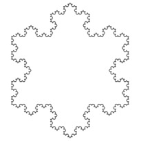
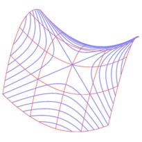
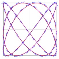
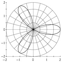
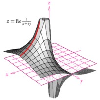
En cliquant sur une imagette, vous accéderez au source et à l'image. En cliquant sur cette dernière, vous ouvrirez le fichier PDF associé.
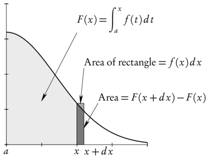
/* -*-ePiX-*- */
/* shadeplot.xp -- February 09, 2003 */
#include "epix.h"
using namespace ePiX;
double k=4;           // change width of hump
double dx = 0.05;     // width of thin shaded region
double x = 1/sqrt(k); // position of thin shaded region
double dy = 0.25;     // for vertical distance between labels; kludgey

double f(double t) { return sqrt(fabs(k)/(2*M_PI))*exp(-k*t*t); }
P pt1 = P(x, f(x)+2*dy), pt2 = P(x+dx,f(x)+dy), pt3 = P(x+3*dx,f(x));

int main()
{
  unitlength("1pt");
  picture(150, 150);
  bounding_box(P(0,0), P(1,1));
  offset(120, -320);

  begin();
  fill();
  gray(0.1);     shadeplot(f, x_min, x, 90);
  gray(0.4);     rect(P(x,f(x)), P(x+dx, 0));
  gray(0.6);     shadeplot(f, x, x+dx, 10);
  fill(false);

  arrow_camber(0.25);  arrow_fill(1);
  arrow(pt1, P(0.5*(x_min+x), 0.5*f(0.5*(x_min+x))),
        P(0,0), "$F(x)=\\displaystyle\\int_a^x f(t)\\,dt$", tr);

  arrow(pt2, P(x+0.5*dx, f(x)),
        P(0,0), "Area of rectangle = $f(x)\\,dx$", tr);

  arrow(pt3, P(x+dx, 0.5*f(x+dx)),
        P(0,0), "Area = $F(x+dx)-F(x)$", tr);

  bold();
  plot(f, x_min, x_max, 120);

  plain(); h_axis(4); v_axis(4);

  label(P(x_min,0), P(0,-5), "$a$", b);
  label(P(x,0), P(0,-5), "$x$", b);
  label(P(x+dx,0), P(0,-2), "$x+dx$", br);

  end();

}